Slopeshade v. Hillshade for bedrock contact mapping

The Digital Dirt Map of Clark County, Nevada is proceeding with a team of 13 now. The goal is to complete the map by May 1 (!), so the team may grow by a couple more members soon. One of the key issues that we are currently grappling with is the refinement of the bedrock-alluvium contact in areas where it is poorly expressed by existing sources. For the most part this includes areas previously mapped at only 1:250,000 scale. Areas previously mapped at smaller scales (1:100,000 and 1:24,000) are far less problematic.

Accurately mapping this contact for a final scale of 1:150,000 for our compilation requires some basic approaches. For one thing, I have been actively training a capable team composed primarily of geography and geology students, so the learning curve isn't too steep.  To discern the primary contact, we have multiple base sources at our disposal (e.g., ASTER, NAIP, ETM) as well as a nice hillshade image of the county based on the 10-m DEM data. This particular base image alone allows for a massive improvement in some of the preexisting geologic linework on the basis of distinguishing predominantly steeply sloping and irregular bedrock outcrops from less steep and generally smoother alluvial, aeolian, and playa deposits. However, applying a manipulative trick that maximizes the value of LiDAR imagery for topographic visualization, it is possible to leverage even the 10-m DEM for better results.

The approach is to develop a slopeshade map. In the case of a slopeshade map, all steep slopes are shaded and all gentle slopes are illuminated....no matter what their aspect. It is essentially an isoshade representation where the sun is shining from all angles at once. 

Here are some examples with the 10-m Clark County data, starting with the hillshade:

Looks nice, no? This is a very pleasing way to present the county in cartographic form.

Here is the slopshade version of the same data:

It is quite stark in comparison, but it conveys the topography in a very useful way. Consider the smaller scale versions of the Arrow Canyon area presented below:

The Hillshade version:

The slopeshade version:

Note how different these two images are. In the case of the slopeshade, no topography is masked by shadow. Every slope is rendered in the same way no matter which direction it faces. In this rendition the primary contact between rock and non-rock is quite clear.

For more examples and an explanation of how easy it is to derive this type of image, check the following links:

http://geofroth.posterous.com/useful-new-lidar-love-tips

http://geofroth.posterous.com/more-lidardifferent-river

Happy mapping!

Posted via email from Fresh Geologic Froth

Nevada Digital Dirt Team undergoes major expansion

Over the past several weeks, I have initiated a major expansion of the Dirt Mapping Team. Completing such a large map by the beginning of May (!) is a mammoth undertaking. As the previous post indicates, we have made significant progress, but it has become clear that the active mapping team was too small (essentially, two of us). The increase in membership has been greatly facilitated through direct cooperation with the affiliated ecosystem mapping and GIS team from the UNR G-lab, and from some 'hand-picked' UNR geology students and profs with skills in mapping and GIS. 


Thus, we now have up to 11 contributors performing at various levels and time commitments. Currently, our main tasks are improving existing linework from compiled map sources and dealing with mapped units that are below our minimum map unit threshold. The first step in the linework improvement phase is modification/reshaping of the contact between bedrock units and surficial units. This turns out to be the easiest step for new 'recruits' to understand and master. The process is greatly enhanced by including multiple imagery types and shaded relief models as base layers which allow for different, yet complementary perspectives on the landscape. Also, running Google Earth in an adjacent monitor is also quite handy. Oh right...the G-Lab also got some sweet new Wacom digitizing tablets as well.


We are using versioned geodatabases in ArcSDE. to allow for independent and concurrent editing among all of us. This is the best scenario for a multi-mapper effort. Thanks to Abbey for managing the whole affair.


The ideal trajectory of mapping participation is as follows:


1. Contact between bedrock and surficial deposits (currently underway)


2. Contact between different master classes of surficial deposits (e.g., alluvial fans from playas, etc.)


3. Contact within master classes of surficial deposits (e.g., alluvial fan deposits of different ages)


Progression through these steps will depend in large part on performance and time available to map. Most team members have been assigned a 15' by 15' (minutes of lat and long) cell in which to work on the bedrock contact. They are tracking their time. Every cell will be evaluated for consistency and accuracy by the team leaders. 


To date, I have spent several hours providing tutorials about the most efficient ways to carry out the bedrock / non-bedrock contact and will spend some more time this week to make sure everyone is up to speed. Also, several times in the last few months I have been able to provide some instuction / explanation in the field about the nature of the deposits we are mapping. 

Generalized map of surficial and bedrock units as of February 2010

The Clark County dirt mapping team will soon expand from 4 to 7 or 8 as we approach a key deadline. The morass of linework remains a major issue, but we are slowly refining it into a clean data set. Here, I thought I would take a step back and evaluate the map on a more fundamental level...that of key mappable unit types. Much of this map reflects the original data sources that we are refining, but it provides a very nice overview of the distribution of the key map unit types in the county. The deposits are not divided by age in this rendition...just process / deposit type.

As the full team begins to take on the county en masse, I will post updates of this particular representation as it evolves.

If you are one of the few that view my Geologic Frothings Blog. Please note that the newest manifestation resides at http://geofroth.org.

Posted via web from Fresh Geologic Froth

Minimum mappable unit blues

I have a tendency to map in great detail...even when it is unwarranted or relates to a largely inconsequential stratigraphic situation. This problem is proportional to the quality of the base imagery that I have or the intrigue-level of the units in the field. However, in my quest to lead the effort to develop a surficial geologic map 10,000 sq. km. of dirt in Clark County in a compressed time frame, I am learning that it is ok not to sweat the details, as long as you explain what comprises the mapped units. One thing that we have learned is that it is essential to develop an agreed-upon minimum map unit area (mmu). That is, the smallest polygon that is mappable at the chosen scale.

As far as I can tell, geologists are not very keen on the mmu, whereas the dirt mappers in the NRCS have codified the concept in their considerably more standardized procedure.

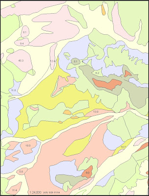
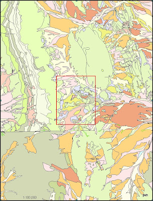
We have adopted a visual approach that is based on the basic legibility of a polygon at a specific scale, and have concluded that 10 hectares is a good minimum value to start with. Ten hectares covers 100,000 square meters...or a square that is approximately 316 meters on a side. Sounds kinda big, looks quite big in the field, and certainly looks mappable at 1:24,000. However, if you zoom out to 1:100,000, the story changes.

The map below shows a random area in the county at 1:24,000. A selection of polygons is labeled with respect to size in hectares.

Sure, those all look totally mappable, right? Well, not so much. Check out the area when outlined in a 100k map:

(note: larger images viewable at:
http://geofroth.posterous.com/minimum-mappable-unit-blues)

Now the story is different. Not only are the small polygons bordering on illegible, the scale of the task of mapping such small polys consistently in a reasonable amount of time is impractical without a huge expenditure of time.

There are some side effects of eliminating units below a certain size threshold. One is data loss. That will be handled by preserving the small polys as points. Thus their locations will be stored as will their attributes. This solution can also facilitate the mapping process by flagging those polys that need to be absorbed into larger, surrounding or adjacent ones. One other problem is the case of high-standing inselbergs. Some of these are very tiny, but protrude several meters above the surrounding surficial deposits. Thus, their omission is particularly notable when in the field. For example, in the photo below, the fairly conspicuous cluster of red sandstone inselbergs has an areal extent of approximately 10 ha.

Not mapping such a feature may seem like a total affront to the sensibility of a geologist, but there will be a point there in the dataset that indicates an awareness of the feature's existence.

More on this later.

Posted via email from Fresh Geologic Froth

Generalized Parent Material Map Progress

We recently generalized the existing bedrock geologic data for Clark County into 19 general lithologic categories. Our goal is to provide clear context for evaluating parent rock materials for the array of surficial deposits that we are compiling and mapping in more detail.

The units have been preliminarily divided into the following 19 categories (2 not yet used on the map):

Sedimentary Rocks (S)

Carbonates (Sc)
Limestone (Scl)
Dolomite (Scd)
Interbedded limestone and dolomite (Scld)

Siliciclastic sedimentary rocks (Ss)
Mudrock and shale (Sssh) (not yet used)
Chert and argillite (Ssc) (not yet used)
Sandstone and coarser (Ssss)
Interbedded shale and sandstone (Ssshss)

Interbedded carbonates and siliciclastic sedimentary rocks (Scs)

Igneous Rocks (I) Plutonic (p) Volcanic (v)

Felsic igneous

Intrusive (granite) (Ipf)
Extrusive (rhyolite and tuff) (Ivf)

Intermediate igneous
Intrusive (diorite) (Ipi)
Extrusive (andesite) (Ivi)

Mafic igneous
Intrusive (gabbro) (Imi)
Extrusive (basalt) (Ivi)

Mixed volcanic rocks (Ivx)

Metamorphic (M)

High grade (crystalline rocks) (Mh)
Low grade (phyllite, argillite, quartzite) (Ml)

It may be that this is more detail than is warranted...or maybe it is not quite enough...opinions will vary. The data are structured in such a way that ratcheting the detail up or down is not complicated. The goal is to work with the existing data in a consistent way across the study area.

Also, note that this project does not involve remapping any bedrock units other than where the boundaries with the Q deposits can be improved.

Correlating units from many maps

We reviewed the nomenclature for the existing maps that cover Clark County and correlated those units to the newly-developed Clark County nomenclature based on deposit type, what materials it is composed of, and any age constraints. In cases where the units do not correlate well, we simply added additional units to the Clark County nomenclature to accommodate the existing map’s nomenclature.

The following maps were compiled:
Las Vegas 100k: usgs sim 05-2814
Lake Mead 100k: usgs ofr 07-1010
Mesquite Lake 100k: usgs ofr 06-1035
Ludington, unpublished data
Death Valley ground-water model area, 250k: usgs mf 2381
Colorado, White River, and Death Valley groundwater flow systems, 250k: nbmg m150


This list of units with brief descriptions is the current Clark County nomenclature.

The following correlation diagrams are split by deposit type and show how all the compiled maps correlate to each other and to the new Clark County nomenclature.